18 Part 1: Dummy Variables and Interaction Effects (Simulation)
18.1 Data Generating Process
Suppose we simulate a study about the effect of a job training program on wages.
Variables:
wage: hourly wagefemale: 1 if femaletraining: 1 if worker attended training programeduc: years of educationtraining_female: interaction between training and female
Interpretation goal: determine whether training increases wages and whether the effect differs by gender.
set.seed(123)

n <- 1000

sim_data <- tibble(
  female = rbinom(n,1,0.5),
  training = rbinom(n,1,0.4),
  educ = round(rnorm(n,12,2))
) %>%
  mutate(
    training_female = training*female,
    wage = 8 +
           0.8*educ +
           1.5*training +
           (-1.0)*female +
           (-0.7)*training_female +
           rnorm(n,0,2)
  )

summary(sim_data)
## female training educ training_female wage
## Min. :0.000 Min. :0.000 Min. : 6.0 Min. :0.000 Min. : 9.502
## 1st Qu.:0.000 1st Qu.:0.000 1st Qu.:11.0 1st Qu.:0.000 1st Qu.:15.747
## Median :0.000 Median :0.000 Median :12.0 Median :0.000 Median :17.502
## Mean :0.493 Mean :0.386 Mean :12.1 Mean :0.172 Mean :17.608
## 3rd Qu.:1.000 3rd Qu.:1.000 3rd Qu.:14.0 3rd Qu.:0.000 3rd Qu.:19.456
## Max. :1.000 Max. :1.000 Max. :19.0 Max. :1.000 Max. :26.28718.2 Regression Model
\(wage = \beta_0 + \beta_1 training + \beta_2 female + \beta_3 (training \cdot female) + \beta_4 educ + u\)
model_sim <- lm(wage ~ training + female + training_female + educ, data = sim_data)
summary(model_sim)
##
## Call:
## lm(formula = wage ~ training + female + training_female + educ,
## data = sim_data)
##
## Residuals:
## Min 1Q Median 3Q Max
## -5.5004 -1.2808 -0.0565 1.3490 6.8218
##
## Coefficients:
## Estimate Std. Error t value Pr(>|t|)
## (Intercept) 7.7616 0.3848 20.169 < 0.0000000000000002 ***
## training 1.2314 0.1761 6.994 0.00000000000488 ***
## female -1.0992 0.1582 -6.950 0.00000000000658 ***
## training_female -0.3404 0.2553 -1.333 0.183
## educ 0.8239 0.0302 27.281 < 0.0000000000000002 ***
## ---
## Signif. codes: 0 '***' 0.001 '**' 0.01 '*' 0.05 '.' 0.1 ' ' 1
##
## Residual standard error: 1.957 on 995 degrees of freedom
## Multiple R-squared: 0.4787, Adjusted R-squared: 0.4766
## F-statistic: 228.4 on 4 and 995 DF, p-value: < 0.0000000000000002218.3 Interpreting Each Coefficient
18.3.1 Intercept
The intercept represents the predicted wage for the reference group.
Reference group here:
male
not in training
education = 0
In practice the intercept is often not that important because zero education may be unrealistic.
18.3.2 Training coefficient
The coefficient on training measures the effect of training for males.
Why?
Because the interaction term allows the effect of training to change for females.
Interpretation example:
“Among males, participation in the training program increases wages by approximately β₁ units on average, holding education constant.”
18.3.3 Female coefficient
The coefficient on female measures the gender wage gap among workers who did not receive training.
Interpretation:
“Among workers without training, females earn β₂ units less than males on average.”
18.3.4 Interaction term
The coefficient on training_female shows how the training effect differs for females relative to males.
Important rule:
Do not interpret this coefficient by itself.
Instead compute the total effect.
Training effect for males: \(\beta_1\)
Training effect for females: \(\beta_1+\beta_3\)
Example interpretation:
“Training increases wages for males by β₁ units, but the training effect for females is β₁ + β₃. The negative interaction coefficient indicates that the training effect is smaller for females.”
18.4 Visualizing Interaction Effects
ggplot(sim_data, aes(x = training, y = wage, color = factor(female)))+
  geom_jitter(alpha=.3)+
  geom_smooth(method="lm", se=FALSE)+
  labs(color="Female")+
  theme_minimal()
## `geom_smooth()` using formula = 'y ~ x'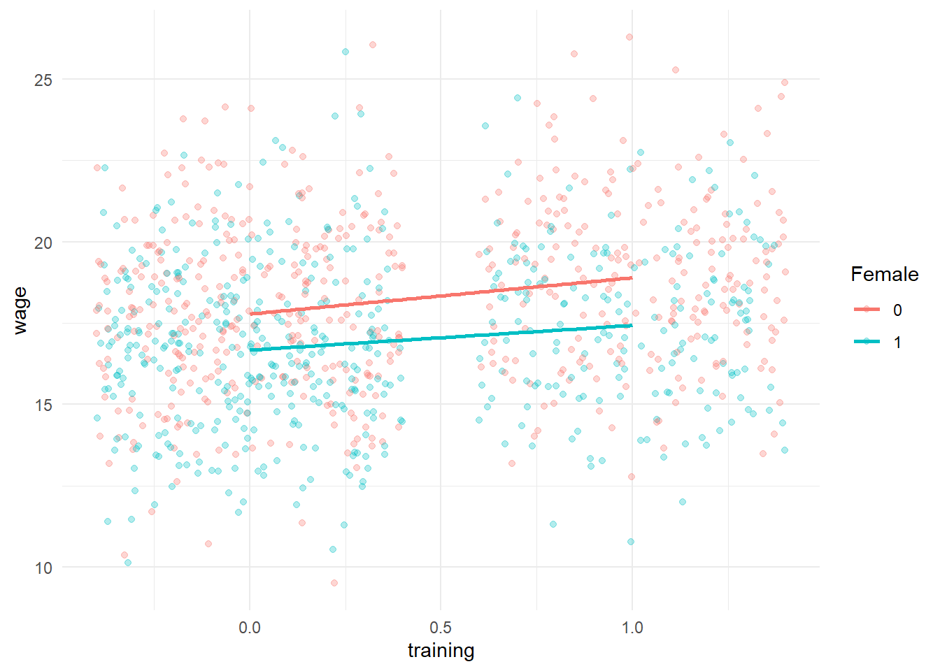
The graph helps visualize that the slope of training differs across groups.