20 Additional Topics

20.1 Preliminaries

20.1.1 Installing and Loading Packages

# Helper function: install if not already installed
if (!require(wooldridge))   install.packages("wooldridge")
if (!require(AER))          install.packages("AER")
if (!require(modelsummary)) install.packages("modelsummary")
if (!require(sandwich))     install.packages("sandwich")
if (!require(lmtest))       install.packages("lmtest")
if (!require(mediation))    install.packages("mediation")
if (!require(margins))      install.packages("margins")
if (!require(plm))          install.packages("plm")
if (!require(samplingbook)) install.packages("samplingbook")
if (!require(psych))        install.packages("psych")
if (!require(igraph))       install.packages("igraph")
if (!require(ggplot2))      install.packages("ggplot2")
if (!require(tidyverse))    install.packages("tidyverse")
if (!require(forecast))     install.packages("forecast")
if (!require(zoo))          install.packages("zoo")
if (!require(tseries))      install.packages("tseries")

library(wooldridge)
library(AER)
library(modelsummary)
library(sandwich)
library(lmtest)
library(mediation)
library(margins)
library(plm)
library(samplingbook)
library(psych)
library(igraph)
library(ggplot2)
library(tidyverse)
library(forecast)
library(zoo)
library(tseries)

20.1.2 Datasets Used in This Lecture

# Wooldridge datasets
data("wage1")   # wages, education, experience, tenure, gender
data("wage2")   # wages with father's education (for IV)
data("mroz")    # female labor force participation

# Panel data
data("Grunfeld") # 10 US firms over 20 years (plm package)

# Base R time series
data("AirPassengers") # monthly airline passengers 1949-1960

# bfi dataset (psych package) - Big Five personality items
data(bfi)

20.2 1. Beginning

\(wage_i=\beta_0+\beta_1 educ_i + u_i\)

The key coefficient is \(\beta_1\). It tells you how much wages change, on average, when education changes by 1 unit.

So if \(\hat{\beta}_1=0.50\), then one extra year of education is associated with 0.50 more units of wage.

The methods to be discussed:

is this relationship causal?
is it stable?
is it the same for everyone?
what happens if the outcome is binary instead of continuous?
what if treatment happens over time?
what if people affect each other through networks?

20.3 2. Causal Inference

20.3.1 Intuition

A beginner often sees a positive coefficient and immediately says: education increases wages. That is too fast. A regression can show that education and wages move together, but that does not automatically mean education caused wages to increase.

Why not?

People with more education may also differ in other ways: richer families, higher ability, more motivation, or better labor markets. If those omitted factors also affect wages, then the regression is mixing up the effect of education with those other factors.

Causal inference asks: What would happen to the same person’s wage if their education changed, holding everything else that matters fixed? That comparison is called the counterfactual idea.

20.3.2 Econometric Idea

Start with a simple model:

\[Y_i = \beta_0 + \beta_1 X_i + u_i\]

OLS works well for causal interpretation only if \(E[u_i \mid X_i] = 0\). This often fails due to omitted variable bias, reverse causality, or selection bias.

20.3.3 Simple and Multiple OLS

names(wage1)

##  [1] "wage"     "educ"     "exper"    "tenure"   "nonwhite" "female"   "married"  "numdep"   "smsa"     "northcen" "south"    "west"    
## [13] "construc" "ndurman"  "trcommpu" "trade"    "services" "profserv" "profocc"  "clerocc"  "servocc"  "lwage"    "expersq"  "tenursq"

model1 <- lm(wage ~ educ, data = wage1)
summary(model1)

## 
## Call:
## lm(formula = wage ~ educ, data = wage1)
## 
## Residuals:
##     Min      1Q  Median      3Q     Max 
## -5.3396 -2.1501 -0.9674  1.1921 16.6085 
## 
## Coefficients:
##             Estimate Std. Error t value            Pr(>|t|)    
## (Intercept) -0.90485    0.68497  -1.321               0.187    
## educ         0.54136    0.05325  10.167 <0.0000000000000002 ***
## ---
## Signif. codes:  0 '***' 0.001 '**' 0.01 '*' 0.05 '.' 0.1 ' ' 1
## 
## Residual standard error: 3.378 on 524 degrees of freedom
## Multiple R-squared:  0.1648, Adjusted R-squared:  0.1632 
## F-statistic: 103.4 on 1 and 524 DF,  p-value: < 0.00000000000000022

model2 <- lm(wage ~ educ + exper + tenure, data = wage1)
summary(model2)

## 
## Call:
## lm(formula = wage ~ educ + exper + tenure, data = wage1)
## 
## Residuals:
##     Min      1Q  Median      3Q     Max 
## -7.6068 -1.7747 -0.6279  1.1969 14.6536 
## 
## Coefficients:
##             Estimate Std. Error t value             Pr(>|t|)    
## (Intercept) -2.87273    0.72896  -3.941   0.0000922474249625 ***
## educ         0.59897    0.05128  11.679 < 0.0000000000000002 ***
## exper        0.02234    0.01206   1.853               0.0645 .  
## tenure       0.16927    0.02164   7.820   0.0000000000000293 ***
## ---
## Signif. codes:  0 '***' 0.001 '**' 0.01 '*' 0.05 '.' 0.1 ' ' 1
## 
## Residual standard error: 3.084 on 522 degrees of freedom
## Multiple R-squared:  0.3064, Adjusted R-squared:  0.3024 
## F-statistic: 76.87 on 3 and 522 DF,  p-value: < 0.00000000000000022

model3 <- lm(log(wage) ~ educ + exper + tenure, data = wage1)
summary(model3)

## 
## Call:
## lm(formula = log(wage) ~ educ + exper + tenure, data = wage1)
## 
## Residuals:
##      Min       1Q   Median       3Q      Max 
## -2.05802 -0.29645 -0.03265  0.28788  1.42809 
## 
## Coefficients:
##             Estimate Std. Error t value             Pr(>|t|)    
## (Intercept) 0.284360   0.104190   2.729              0.00656 ** 
## educ        0.092029   0.007330  12.555 < 0.0000000000000002 ***
## exper       0.004121   0.001723   2.391              0.01714 *  
## tenure      0.022067   0.003094   7.133     0.00000000000329 ***
## ---
## Signif. codes:  0 '***' 0.001 '**' 0.01 '*' 0.05 '.' 0.1 ' ' 1
## 
## Residual standard error: 0.4409 on 522 degrees of freedom
## Multiple R-squared:  0.316,  Adjusted R-squared:  0.3121 
## F-statistic: 80.39 on 3 and 522 DF,  p-value: < 0.00000000000000022

Reading the output: If the coefficient on educ is 0.09 in a log-wage model, it means that holding experience and tenure constant, one additional year of education is associated with about an 9% higher wage.

20.3.4 Instrumental Variables

An instrument \(Z\) must satisfy two conditions:

Relevance — it must affect the endogenous variable \(X\)
Exogeneity / exclusion restriction — it must affect \(Y\) only through \(X\), not directly

# OLS first
ols_iv <- lm(log(wage) ~ educ + exper + tenure, data = wage2)
summary(ols_iv)

## 
## Call:
## lm(formula = log(wage) ~ educ + exper + tenure, data = wage2)
## 
## Residuals:
##     Min      1Q  Median      3Q     Max 
## -1.8282 -0.2401  0.0203  0.2569  1.3400 
## 
## Coefficients:
##             Estimate Std. Error t value             Pr(>|t|)    
## (Intercept) 5.496696   0.110528  49.731 < 0.0000000000000002 ***
## educ        0.074864   0.006512  11.495 < 0.0000000000000002 ***
## exper       0.015328   0.003370   4.549          0.000006100 ***
## tenure      0.013375   0.002587   5.170          0.000000287 ***
## ---
## Signif. codes:  0 '***' 0.001 '**' 0.01 '*' 0.05 '.' 0.1 ' ' 1
## 
## Residual standard error: 0.3877 on 931 degrees of freedom
## Multiple R-squared:  0.1551, Adjusted R-squared:  0.1524 
## F-statistic: 56.97 on 3 and 931 DF,  p-value: < 0.00000000000000022

# IV using father's education (feduc) as instrument for educ
iv_model <- ivreg(log(wage) ~ educ + exper + tenure |
                    feduc + exper + tenure,
                  data = wage2)
summary(iv_model)

## 
## Call:
## ivreg(formula = log(wage) ~ educ + exper + tenure | feduc + exper + 
##     tenure, data = wage2)
## 
## Residuals:
##       Min        1Q    Median        3Q       Max 
## -1.712589 -0.248278  0.007354  0.269977  1.356545 
## 
## Coefficients:
##             Estimate Std. Error t value             Pr(>|t|)    
## (Intercept) 4.435860   0.338928  13.088 < 0.0000000000000002 ***
## educ        0.140255   0.020804   6.742      0.0000000000316 ***
## exper       0.035152   0.006307   5.574      0.0000000350183 ***
## tenure      0.007409   0.003186   2.325               0.0203 *  
## ---
## Signif. codes:  0 '***' 0.001 '**' 0.01 '*' 0.05 '.' 0.1 ' ' 1
## 
## Residual standard error: 0.4075 on 737 degrees of freedom
## Multiple R-Squared: 0.05179, Adjusted R-squared: 0.04793 
## Wald test: 21.42 on 3 and 737 DF,  p-value: 0.0000000000002593

# Diagnostics
summary(iv_model, diagnostics = TRUE)

## 
## Call:
## ivreg(formula = log(wage) ~ educ + exper + tenure | feduc + exper + 
##     tenure, data = wage2)
## 
## Residuals:
##       Min        1Q    Median        3Q       Max 
## -1.712589 -0.248278  0.007354  0.269977  1.356545 
## 
## Coefficients:
##             Estimate Std. Error t value             Pr(>|t|)    
## (Intercept) 4.435860   0.338928  13.088 < 0.0000000000000002 ***
## educ        0.140255   0.020804   6.742      0.0000000000316 ***
## exper       0.035152   0.006307   5.574      0.0000000350183 ***
## tenure      0.007409   0.003186   2.325               0.0203 *  
## 
## Diagnostic tests:
##                  df1 df2 statistic              p-value    
## Weak instruments   1 737    110.32 < 0.0000000000000002 ***
## Wu-Hausman         1 736     13.06             0.000322 ***
## Sargan             0  NA        NA                   NA    
## ---
## Signif. codes:  0 '***' 0.001 '**' 0.01 '*' 0.05 '.' 0.1 ' ' 1
## 
## Residual standard error: 0.4075 on 737 degrees of freedom
## Multiple R-Squared: 0.05179, Adjusted R-squared: 0.04793 
## Wald test: 21.42 on 3 and 737 DF,  p-value: 0.0000000000002593

Note: IV often estimates a local effect: meaning, only for the group whose education is affected by the instrument. The coefficient can differ substantially from OLS.

20.3.5 Common Mistakes

Calling OLS causal without discussion
- meaning a positive OLS is not enough
Ignoring omitted variables like ability or family background
- because coefficient can be biased
Treating “holding other variables constant” as the same as causal
- not the same
Using IV without defending relevance and exogeneity
Thinking more controls always solve endogeneity

20.4 3. Robustness Checks

20.4.1 Intuition

A result is fragile if it disappears when you add a few controls, use robust standard errors, change the functional form, or restrict the sample. Robustness checks ask: Does my conclusion still hold under reasonable alternative modeling choices?

20.4.2 Gradual Addition of Controls

robust1 <- lm(log(wage) ~ educ, data = wage1)
summary(robust1)

## 
## Call:
## lm(formula = log(wage) ~ educ, data = wage1)
## 
## Residuals:
##      Min       1Q   Median       3Q      Max 
## -2.21158 -0.36393 -0.07263  0.29712  1.52339 
## 
## Coefficients:
##             Estimate Std. Error t value             Pr(>|t|)    
## (Intercept) 0.583773   0.097336   5.998        0.00000000374 ***
## educ        0.082744   0.007567  10.935 < 0.0000000000000002 ***
## ---
## Signif. codes:  0 '***' 0.001 '**' 0.01 '*' 0.05 '.' 0.1 ' ' 1
## 
## Residual standard error: 0.4801 on 524 degrees of freedom
## Multiple R-squared:  0.1858, Adjusted R-squared:  0.1843 
## F-statistic: 119.6 on 1 and 524 DF,  p-value: < 0.00000000000000022

robust2 <- lm(log(wage) ~ educ + exper + tenure, data = wage1)
summary(robust2)

## 
## Call:
## lm(formula = log(wage) ~ educ + exper + tenure, data = wage1)
## 
## Residuals:
##      Min       1Q   Median       3Q      Max 
## -2.05802 -0.29645 -0.03265  0.28788  1.42809 
## 
## Coefficients:
##             Estimate Std. Error t value             Pr(>|t|)    
## (Intercept) 0.284360   0.104190   2.729              0.00656 ** 
## educ        0.092029   0.007330  12.555 < 0.0000000000000002 ***
## exper       0.004121   0.001723   2.391              0.01714 *  
## tenure      0.022067   0.003094   7.133     0.00000000000329 ***
## ---
## Signif. codes:  0 '***' 0.001 '**' 0.01 '*' 0.05 '.' 0.1 ' ' 1
## 
## Residual standard error: 0.4409 on 522 degrees of freedom
## Multiple R-squared:  0.316,  Adjusted R-squared:  0.3121 
## F-statistic: 80.39 on 3 and 522 DF,  p-value: < 0.00000000000000022

robust3 <- lm(log(wage) ~ educ + exper + tenure + female + married, data = wage1)
summary(robust3)

## 
## Call:
## lm(formula = log(wage) ~ educ + exper + tenure + female + married, 
##     data = wage1)
## 
## Residuals:
##      Min       1Q   Median       3Q      Max 
## -1.87254 -0.27256 -0.03779  0.25349  1.23666 
## 
## Coefficients:
##              Estimate Std. Error t value             Pr(>|t|)    
## (Intercept)  0.490058   0.101108   4.847     0.00000165830384 ***
## educ         0.083905   0.006973  12.033 < 0.0000000000000002 ***
## exper        0.003134   0.001682   1.863              0.06300 .  
## tenure       0.016867   0.002955   5.707     0.00000001932029 ***
## female      -0.285530   0.037264  -7.662     0.00000000000009 ***
## married      0.125739   0.039986   3.145              0.00176 ** 
## ---
## Signif. codes:  0 '***' 0.001 '**' 0.01 '*' 0.05 '.' 0.1 ' ' 1
## 
## Residual standard error: 0.4125 on 520 degrees of freedom
## Multiple R-squared:  0.4036, Adjusted R-squared:  0.3979 
## F-statistic: 70.38 on 5 and 520 DF,  p-value: < 0.00000000000000022

20.4.3 Side-by-Side Comparison

If you don’t want stargazer, we can make a list and it will appear as a good table too. It will appear in the Viewer too:

modelsummary(list(
  "Simple"               = robust1,
  "Exp + Tenure"         = robust2,
  "Add Demographics"     = robust3
))

	Simple	Exp + Tenure	Add Demographics
(Intercept)	0.584	0.284	0.490
	(0.097)	(0.104)	(0.101)
educ	0.083	0.092	0.084
	(0.008)	(0.007)	(0.007)
exper		0.004	0.003
		(0.002)	(0.002)
tenure		0.022	0.017
		(0.003)	(0.003)
female			-0.286
			(0.037)
married			0.126
			(0.040)
Num.Obs.	526	526	526
R2	0.186	0.316	0.404
R2 Adj.	0.184	0.312	0.398
AIC	2432.4	2344.8	2276.7
BIC	2445.2	2366.1	2306.5
Log.Lik.	-359.378	-313.548	-277.505
F	119.582	80.391	70.383
RMSE	0.48	0.44	0.41

20.4.4 Heteroskedasticity-Robust Standard Errors

Robust SEs do not change the coefficients — only the standard errors, t-statistics, and p-values.

coeftest(robust2, vcov = vcovHC(robust2, type = "HC1"))

## 
## t test of coefficients:
## 
##              Estimate Std. Error t value              Pr(>|t|)    
## (Intercept) 0.2843596  0.1117069  2.5456               0.01120 *  
## educ        0.0920290  0.0079212 11.6181 < 0.00000000000000022 ***
## exper       0.0041211  0.0017459  2.3605               0.01862 *  
## tenure      0.0220672  0.0037820  5.8348        0.000000009461 ***
## ---
## Signif. codes:  0 '***' 0.001 '**' 0.01 '*' 0.05 '.' 0.1 ' ' 1

20.4.5 Nonlinear Specification

robust4 <- lm(log(wage) ~ educ + exper + I(exper^2) + tenure, data = wage1)
summary(robust4)

## 
## Call:
## lm(formula = log(wage) ~ educ + exper + I(exper^2) + tenure, 
##     data = wage1)
## 
## Residuals:
##      Min       1Q   Median       3Q      Max 
## -1.97087 -0.26809 -0.03463  0.27663  1.28678 
## 
## Coefficients:
##               Estimate Std. Error t value             Pr(>|t|)    
## (Intercept)  0.1983445  0.1019556   1.945               0.0523 .  
## educ         0.0853489  0.0071885  11.873 < 0.0000000000000002 ***
## exper        0.0328542  0.0051135   6.425      0.0000000002979 ***
## I(exper^2)  -0.0006606  0.0001111  -5.945      0.0000000050775 ***
## tenure       0.0208413  0.0030037   6.938      0.0000000000118 ***
## ---
## Signif. codes:  0 '***' 0.001 '**' 0.01 '*' 0.05 '.' 0.1 ' ' 1
## 
## Residual standard error: 0.427 on 521 degrees of freedom
## Multiple R-squared:  0.3595, Adjusted R-squared:  0.3545 
## F-statistic: 73.09 on 4 and 521 DF,  p-value: < 0.00000000000000022

20.4.6 Trimming Outliers

summary(wage1$wage)

##    Min. 1st Qu.  Median    Mean 3rd Qu.    Max. 
##   0.530   3.330   4.650   5.896   6.880  24.980

quantile(wage1$wage, probs = c(0.95, 0.99))

##    95%    99% 
## 12.875 19.995

trim_data <- subset(wage1, wage < quantile(wage, 0.99))
robust5 <- lm(log(wage) ~ educ + exper + tenure, data = trim_data)
summary(robust5)

## 
## Call:
## lm(formula = log(wage) ~ educ + exper + tenure, data = trim_data)
## 
## Residuals:
##      Min       1Q   Median       3Q      Max 
## -2.05464 -0.29310 -0.02882  0.28405  1.23528 
## 
## Coefficients:
##             Estimate Std. Error t value             Pr(>|t|)    
## (Intercept) 0.319145   0.101333   3.149              0.00173 ** 
## educ        0.089004   0.007142  12.462 < 0.0000000000000002 ***
## exper       0.004014   0.001666   2.410              0.01631 *  
## tenure      0.020525   0.003016   6.805      0.0000000000282 ***
## ---
## Signif. codes:  0 '***' 0.001 '**' 0.01 '*' 0.05 '.' 0.1 ' ' 1
## 
## Residual standard error: 0.4258 on 516 degrees of freedom
## Multiple R-squared:  0.3072, Adjusted R-squared:  0.3032 
## F-statistic: 76.27 on 3 and 516 DF,  p-value: < 0.00000000000000022

20.4.7 How to read the output

When doing robustness checks, do not read each regression separately as if it were a stand-alone project. Instead, compare across models.

Ask these questions:

Does the sign stay the same?
- If education is positive in all models, that is reassuring.

Does the size stay broadly similar?
- If the coefficient moves from 0.10 to 0.08 to 0.07, that is usually acceptable.
- If it moves from 0.10 to -0.03, that is a major warning sign.

Does the result stay statistically meaningful?
- If the coefficient remains precisely estimated under robust standard errors and alternative specifications, that strengthens confidence.
Does the economic interpretation stay similar?
- Even if the exact coefficient changes a bit, does the basic story remain the same?
- For example:
  - Model 1: 10% return to education
  - Model 2: 8% return
  - Model 3: 7% return

You would say:

The estimated return to education falls somewhat when additional controls are included, suggesting that part of the raw education-wage relationship reflects other factors. However, the coefficient remains positive and economically meaningful across specifications.

20.4.8 Common Mistakes

Treating robustness checks as optional
Looking only at significance, ignoring magnitude
Hiding models that contradict your preferred result
Changing the model randomly without economic justification

20.5 4. Heterogeneity Analysis

20.5.1 Intuition

A single average effect may hide important differences across groups. Does the effect of education on wages differ by gender? This is heterogeneity.

20.5.2 Econometric Idea

\[Y = \beta_0 + \beta_1 X + \beta_2 G + \beta_3 (X \times G) + u\]

\(\beta_1\) = effect of \(X\) for the baseline group (\(G = 0\))
\(\beta_3\) = difference in slope between groups (not the full effect for the second group)
Effect for women: \(\beta_1 + \beta_3\)

20.5.3 Interaction Model

het1 <- lm(log(wage) ~ educ * female + exper + tenure, data = wage1)
summary(het1)

## 
## Call:
## lm(formula = log(wage) ~ educ * female + exper + tenure, data = wage1)
## 
## Residuals:
##      Min       1Q   Median       3Q      Max 
## -1.91695 -0.26530 -0.02059  0.25715  1.27586 
## 
## Coefficients:
##              Estimate Std. Error t value             Pr(>|t|)    
## (Intercept)  0.464712   0.122892   3.781             0.000174 ***
## educ         0.090276   0.008715  10.359 < 0.0000000000000002 ***
## female      -0.210376   0.173969  -1.209             0.227107    
## exper        0.004642   0.001628   2.850             0.004541 ** 
## tenure       0.017436   0.002981   5.849        0.00000000876 ***
## educ:female -0.007245   0.013562  -0.534             0.593456    
## ---
## Signif. codes:  0 '***' 0.001 '**' 0.01 '*' 0.05 '.' 0.1 ' ' 1
## 
## Residual standard error: 0.4162 on 520 degrees of freedom
## Multiple R-squared:  0.3926, Adjusted R-squared:  0.3868 
## F-statistic: 67.22 on 5 and 520 DF,  p-value: < 0.00000000000000022

This is equivalent to:

het2 <- lm(log(wage) ~ educ + female + educ:female + exper + tenure, data = wage1)
summary(het2)

## 
## Call:
## lm(formula = log(wage) ~ educ + female + educ:female + exper + 
##     tenure, data = wage1)
## 
## Residuals:
##      Min       1Q   Median       3Q      Max 
## -1.91695 -0.26530 -0.02059  0.25715  1.27586 
## 
## Coefficients:
##              Estimate Std. Error t value             Pr(>|t|)    
## (Intercept)  0.464712   0.122892   3.781             0.000174 ***
## educ         0.090276   0.008715  10.359 < 0.0000000000000002 ***
## female      -0.210376   0.173969  -1.209             0.227107    
## exper        0.004642   0.001628   2.850             0.004541 ** 
## tenure       0.017436   0.002981   5.849        0.00000000876 ***
## educ:female -0.007245   0.013562  -0.534             0.593456    
## ---
## Signif. codes:  0 '***' 0.001 '**' 0.01 '*' 0.05 '.' 0.1 ' ' 1
## 
## Residual standard error: 0.4162 on 520 degrees of freedom
## Multiple R-squared:  0.3926, Adjusted R-squared:  0.3868 
## F-statistic: 67.22 on 5 and 520 DF,  p-value: < 0.00000000000000022

20.5.4 Separate Subgroup Regressions

male_model   <- lm(log(wage) ~ educ + exper + tenure, data = subset(wage1, female == 0))
female_model <- lm(log(wage) ~ educ + exper + tenure, data = subset(wage1, female == 1))

summary(male_model)

## 
## Call:
## lm(formula = log(wage) ~ educ + exper + tenure, data = subset(wage1, 
##     female == 0))
## 
## Residuals:
##     Min      1Q  Median      3Q     Max 
## -1.4849 -0.2784 -0.0103  0.2665  1.2670 
## 
## Coefficients:
##             Estimate Std. Error t value             Pr(>|t|)    
## (Intercept) 0.321899   0.139460   2.308              0.02174 *  
## educ        0.096264   0.009352  10.294 < 0.0000000000000002 ***
## exper       0.008127   0.002496   3.256              0.00128 ** 
## tenure      0.018213   0.003769   4.832           0.00000227 ***
## ---
## Signif. codes:  0 '***' 0.001 '**' 0.01 '*' 0.05 '.' 0.1 ' ' 1
## 
## Residual standard error: 0.4284 on 270 degrees of freedom
## Multiple R-squared:  0.3655, Adjusted R-squared:  0.3584 
## F-statistic: 51.84 on 3 and 270 DF,  p-value: < 0.00000000000000022

summary(female_model)

## 
## Call:
## lm(formula = log(wage) ~ educ + exper + tenure, data = subset(wage1, 
##     female == 1))
## 
## Residuals:
##      Min       1Q   Median       3Q      Max 
## -1.96850 -0.23365 -0.06671  0.21956  1.17698 
## 
## Coefficients:
##             Estimate Std. Error t value          Pr(>|t|)    
## (Intercept) 0.356116   0.141063   2.525            0.0122 *  
## educ        0.080036   0.010462   7.650 0.000000000000444 ***
## exper       0.002268   0.002105   1.077            0.2823    
## tenure      0.010274   0.005223   1.967            0.0503 .  
## ---
## Signif. codes:  0 '***' 0.001 '**' 0.01 '*' 0.05 '.' 0.1 ' ' 1
## 
## Residual standard error: 0.3967 on 248 degrees of freedom
## Multiple R-squared:  0.2119, Adjusted R-squared:  0.2024 
## F-statistic: 22.23 on 3 and 248 DF,  p-value: 0.0000000000008771

Reading the output:

Identify the baseline group
Interpret educ
Interpret educ:female
Compute the education effect for women
Interpret female

20.5.5 Heterogeneity with a Continuous Moderator

Sometimes the effect changes continuously with another variable, such as income.

set.seed(42)
df_het <- data.frame(
  treatment = rbinom(300, 1, 0.5),
  income    = rnorm(300, 50000, 10000)
)
df_het$y <- 10 + 2 * df_het$treatment +
  0.0001 * df_het$income -
  0.00005 * df_het$treatment * df_het$income +
  rnorm(300)

het_cont <- lm(y ~ treatment * income, data = df_het)
summary(het_cont)

## 
## Call:
## lm(formula = y ~ treatment * income, data = df_het)
## 
## Residuals:
##     Min      1Q  Median      3Q     Max 
## -2.9386 -0.6412  0.0113  0.7243  3.3772 
## 
## Coefficients:
##                      Estimate   Std. Error t value             Pr(>|t|)    
## (Intercept)      10.133329521  0.466720653  21.712 < 0.0000000000000002 ***
## treatment         2.133953801  0.626572403   3.406             0.000751 ***
## income            0.000094815  0.000009197  10.309 < 0.0000000000000002 ***
## treatment:income -0.000050444  0.000012353  -4.084            0.0000571 ***
## ---
## Signif. codes:  0 '***' 0.001 '**' 0.01 '*' 0.05 '.' 0.1 ' ' 1
## 
## Residual standard error: 1.002 on 296 degrees of freedom
## Multiple R-squared:  0.332,  Adjusted R-squared:  0.3252 
## F-statistic: 49.03 on 3 and 296 DF,  p-value: < 0.00000000000000022

The treatment effect is \(\frac{\partial y}{\partial \text{treatment}} = \beta_1 + \beta_3 \cdot \text{income}\).

Interpretation:

treatment is the treatment effect when income is zero

treatment:income shows how the treatment effect changes as income rises

20.5.6 Common Mistakes

Interpreting the interaction coefficient as the subgroup effect (it is the difference)
Forgetting to add coefficients when computing the non-baseline group’s effect
Running separate regressions and assuming differences without formally testing them

20.6 5. Moderation Analysis

20.6.1 Intuition

Moderation asks: Does the effect of X on Y depend on another variable (the moderator)?

Examples: Does education matter more in urban areas? Does training help more for younger workers?

20.6.2 Econometric Idea

\[Y = \beta_0 + \beta_1 X + \beta_2 M + \beta_3 (X \times M) + u\]

\[\frac{\partial Y}{\partial X} = \beta_1 + \beta_3 M\]

The slope of \(X\) is not fixed — it depends on the value of the moderator.

20.6.3 R Code

set.seed(1)
df_mod <- data.frame(
  x         = rnorm(300),
  moderator = rnorm(300)
)
df_mod$y <- 1 + 2 * df_mod$x + 1.5 * df_mod$moderator +
  3 * (df_mod$x * df_mod$moderator) + rnorm(300)

mod_model <- lm(y ~ x * moderator, data = df_mod)
summary(mod_model)

## 
## Call:
## lm(formula = y ~ x * moderator, data = df_mod)
## 
## Residuals:
##      Min       1Q   Median       3Q      Max 
## -2.90475 -0.80807  0.02178  0.78318  3.09584 
## 
## Coefficients:
##             Estimate Std. Error t value            Pr(>|t|)    
## (Intercept)  0.93750    0.06305   14.87 <0.0000000000000002 ***
## x            2.03920    0.06610   30.85 <0.0000000000000002 ***
## moderator    1.54063    0.06047   25.48 <0.0000000000000002 ***
## x:moderator  2.93700    0.05906   49.73 <0.0000000000000002 ***
## ---
## Signif. codes:  0 '***' 0.001 '**' 0.01 '*' 0.05 '.' 0.1 ' ' 1
## 
## Residual standard error: 1.091 on 296 degrees of freedom
## Multiple R-squared:  0.9261, Adjusted R-squared:  0.9254 
## F-statistic:  1237 on 3 and 296 DF,  p-value: < 0.00000000000000022

Reading the output: If x = 2.0 and x:moderator = 3.0, then:

When moderator = 0: effect of x = 2
When moderator = 1: effect of x = 5
When moderator = −1: effect of x = −1

20.6.4 Visualization

df_mod$high_mod <- ifelse(df_mod$moderator > 0, 1, 0)

ggplot(df_mod, aes(x = x, y = y, color = factor(high_mod))) +
  geom_point(alpha = 0.5) +
  geom_smooth(method = "lm", se = FALSE) +
  labs(title = "Moderation: Effect of X by Moderator Level",
       color = "High Moderator")

## `geom_smooth()` using formula = 'y ~ x'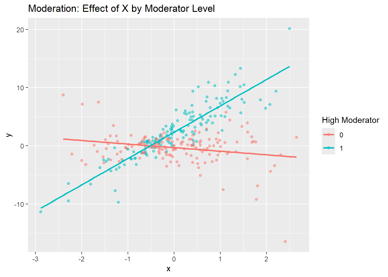

20.6.5 Common Mistakes

Interpreting x as the effect for everyone (it is only when the moderator equals zero)
Describing the interaction but never computing actual slopes at different moderator values

20.7 6. Mediation Analysis

20.7.1 Intuition

Mediation asks not only Does X affect Y? but also Through what channel? This separates the total effect into a direct effect and an indirect effect through a mediator.

20.7.2 Econometric Idea

Two equations:

\(M = \alpha_0 + \alpha_1 X + u\) — does X affect the mediator?
\(Y = \beta_0 + \beta_1 X + \beta_2 M + v\) — does the mediator affect Y, controlling for X?

If education affects skills, and skills affect wages, then part of education’s effect on wages is mediated through skills.

Key quantities: ACME: Average Causal Mediation Effect (indirect effect), ADE: Average Direct Effect (direct effect), Total Effect.

20.7.3 R Code

set.seed(1)
df_med     <- data.frame(x = rnorm(400))
df_med$m   <- 0.6 * df_med$x + rnorm(400) #mediator
df_med$y   <- 1.0 * df_med$x + 2.0 * df_med$m + rnorm(400)

med_model_m <- lm(m ~ x, data = df_med)
summary(med_model_m)

## 
## Call:
## lm(formula = m ~ x, data = df_med)
## 
## Residuals:
##     Min      1Q  Median      3Q     Max 
## -2.9132 -0.7443 -0.0463  0.7516  3.8310 
## 
## Coefficients:
##             Estimate Std. Error t value            Pr(>|t|)    
## (Intercept) -0.07197    0.05407  -1.331               0.184    
## x            0.63230    0.05579  11.333 <0.0000000000000002 ***
## ---
## Signif. codes:  0 '***' 0.001 '**' 0.01 '*' 0.05 '.' 0.1 ' ' 1
## 
## Residual standard error: 1.08 on 398 degrees of freedom
## Multiple R-squared:  0.244,  Adjusted R-squared:  0.2421 
## F-statistic: 128.4 on 1 and 398 DF,  p-value: < 0.00000000000000022

med_model_y <- lm(y ~ x + m, data = df_med) #does the mediator predict y after controlling for x?
summary(med_model_y)

## 
## Call:
## lm(formula = y ~ x + m, data = df_med)
## 
## Residuals:
##     Min      1Q  Median      3Q     Max 
## -3.1768 -0.7045  0.0151  0.7333  3.0897 
## 
## Coefficients:
##             Estimate Std. Error t value            Pr(>|t|)    
## (Intercept) -0.03675    0.05222  -0.704               0.482    
## x            1.00046    0.06184  16.179 <0.0000000000000002 ***
## m            2.00610    0.04831  41.529 <0.0000000000000002 ***
## ---
## Signif. codes:  0 '***' 0.001 '**' 0.01 '*' 0.05 '.' 0.1 ' ' 1
## 
## Residual standard error: 1.041 on 397 degrees of freedom
## Multiple R-squared:  0.8983, Adjusted R-squared:  0.8978 
## F-statistic:  1753 on 2 and 397 DF,  p-value: < 0.00000000000000022

med_out <- mediation::mediate(med_model_m, med_model_y, #we use the mediation package
                   treat    = "x",
                   mediator = "m",
                   boot     = TRUE,
                   sims     = 500)

## Running nonparametric bootstrap

summary(med_out)

## 
## Causal Mediation Analysis 
## 
## Nonparametric Bootstrap Confidence Intervals with the Percentile Method
## 
##                Estimate 95% CI Lower 95% CI Upper               p-value    
## ACME            1.26846      1.04275      1.50707 < 0.00000000000000022 ***
## ADE             1.00046      0.87873      1.12612 < 0.00000000000000022 ***
## Total Effect    2.26891      2.02710      2.52811 < 0.00000000000000022 ***
## Prop. Mediated  0.55906      0.49996      0.61636 < 0.00000000000000022 ***
## ---
## Signif. codes:  0 '***' 0.001 '**' 0.01 '*' 0.05 '.' 0.1 ' ' 1
## 
## Sample Size Used: 400 
## 
## 
## Simulations: 500

Interpretation example:

ACME

This is the indirect effect through the mediator.

If ACME is positive and meaningful, then part of the effect of x on y flows through m.

This is the direct effect of x on y that is not going through m.

Total Effect

This is the overall effect of x on y.

Proportion mediated

This tells you what share of the total effect is explained by the mediator.

If ACME = 1.1, ADE = 0.8, Total = 1.9, then about 1.1 units of the effect of X on Y flow through the mediator, and 0.8 units operate through other channels.

20.7.4 Important Caution

Mediation relies on strong assumptions. A careful statement is: “The mediation analysis is consistent with part of the effect operating through the proposed channel, under the assumptions of the mediation framework.”

20.7.5 Common Mistakes:

Treating mediation as automatic proof of mechanism
Forgetting to model the mediator carefully
Interpreting the proportion too literally

20.8 7. Logistic Regression

20.8.1 Intuition

When the dependent variable is binary (employed / not employed, participates / does not), OLS is not ideal because predicted values can fall outside [0, 1]. Logistic regression models probabilities appropriately.

20.8.2 Econometric Idea

\[P(Y = 1 \mid X) = \frac{1}{1 + e^{-X\beta}}\]

Raw coefficients describe changes in log-odds, not probabilities. Focus on marginal effects and predicted probabilities for interpretation.

20.8.3 R Code

names(mroz)

##  [1] "inlf"     "hours"    "kidslt6"  "kidsge6"  "age"      "educ"     "wage"     "repwage"  "hushrs"   "husage"   "huseduc"  "huswage" 
## [13] "faminc"   "mtr"      "motheduc" "fatheduc" "unem"     "city"     "exper"    "nwifeinc" "lwage"    "expersq"

logit1 <- glm(inlf ~ educ + exper + age + kidslt6, #generalized linear model
              data   = mroz,
              family = binomial(link = "logit")) #sets logistic regression
summary(logit1)

## 
## Call:
## glm(formula = inlf ~ educ + exper + age + kidslt6, family = binomial(link = "logit"), 
##     data = mroz)
## 
## Coefficients:
##             Estimate Std. Error z value             Pr(>|z|)    
## (Intercept)  1.31195    0.73482   1.785               0.0742 .  
## educ         0.18824    0.03997   4.710   0.0000024815263609 ***
## exper        0.12403    0.01319   9.401 < 0.0000000000000002 ***
## age         -0.09984    0.01328  -7.518   0.0000000000000555 ***
## kidslt6     -1.44603    0.19836  -7.290   0.0000000000003101 ***
## ---
## Signif. codes:  0 '***' 0.001 '**' 0.01 '*' 0.05 '.' 0.1 ' ' 1
## 
## (Dispersion parameter for binomial family taken to be 1)
## 
##     Null deviance: 1029.75  on 752  degrees of freedom
## Residual deviance:  818.94  on 748  degrees of freedom
## AIC: 828.94
## 
## Number of Fisher Scoring iterations: 4

# Predicted probabilities
pred_probs <- predict(logit1, type = "response")
head(pred_probs)

##         1         2         3         4         5         6 
## 0.6607172 0.7677956 0.6203450 0.7151622 0.5682189 0.9065924

# Marginal effects
logit_mfx <- margins(logit1)
summary(logit_mfx)

##   factor     AME     SE       z      p   lower   upper
##      age -0.0183 0.0021 -8.7609 0.0000 -0.0224 -0.0142
##     educ  0.0345 0.0069  4.9640 0.0000  0.0208  0.0481
##    exper  0.0227 0.0019 12.1384 0.0000  0.0190  0.0264
##  kidslt6 -0.2646 0.0315 -8.4084 0.0000 -0.3263 -0.2030

# Odds ratios
exp(coef(logit1))

## (Intercept)        educ       exper         age     kidslt6 
##   3.7133901   1.2071263   1.1320524   0.9049849   0.2355033

Reading the output:

Raw coefficient — change in log-odds (not directly interpretable as probability)
Odds ratio — if exp(coef) for education is 1.10, the odds increase by ~10%
- one more year of education multiplies the odds of labor force participation by 1.10 which means the odds increase by about 10%
Marginal effect — if AME for educ is 0.03, one more year of education raises the probability of labor force participation by ~3 percentage points on average
Predicted probability - If a woman has predicted probability 0.72 means estimated probability of being in the labor force is 72%.

20.8.4 Common Mistakes

Interpreting raw coefficients as probability changes
Forgetting to report marginal effects or predicted probabilities
Ignoring the nonlinear nature of the model

20.9 8. Probit Regression

20.9.1 Intuition

Probit solves the same problem as logit but uses the normal CDF instead of the logistic CDF. In practice, logit and probit usually give similar conclusions.

20.9.2 R Code

probit1 <- glm(inlf ~ educ + exper + age + kidslt6,
               data   = mroz,
               family = binomial(link = "probit"))
summary(probit1)

## 
## Call:
## glm(formula = inlf ~ educ + exper + age + kidslt6, family = binomial(link = "probit"), 
##     data = mroz)
## 
## Coefficients:
##             Estimate Std. Error z value             Pr(>|z|)    
## (Intercept)  0.85818    0.43586   1.969                0.049 *  
## educ         0.11170    0.02341   4.771  0.00000183050189589 ***
## exper        0.07289    0.00741   9.836 < 0.0000000000000002 ***
## age         -0.06080    0.00769  -7.906  0.00000000000000266 ***
## kidslt6     -0.87825    0.11551  -7.603  0.00000000000002889 ***
## ---
## Signif. codes:  0 '***' 0.001 '**' 0.01 '*' 0.05 '.' 0.1 ' ' 1
## 
## (Dispersion parameter for binomial family taken to be 1)
## 
##     Null deviance: 1029.75  on 752  degrees of freedom
## Residual deviance:  818.82  on 748  degrees of freedom
## AIC: 828.82
## 
## Number of Fisher Scoring iterations: 4

probit_mfx   <- margins(probit1)
summary(probit_mfx)

##   factor     AME     SE       z      p   lower   upper
##      age -0.0187 0.0021 -9.0329 0.0000 -0.0228 -0.0147
##     educ  0.0344 0.0069  4.9811 0.0000  0.0208  0.0479
##    exper  0.0224 0.0018 12.2454 0.0000  0.0188  0.0260
##  kidslt6 -0.2703 0.0315 -8.5901 0.0000 -0.3319 -0.2086

probit_probs <- predict(probit1, type = "response")
head(probit_probs)

##         1         2         3         4         5         6 
## 0.6536409 0.7700535 0.6124299 0.7152241 0.5671615 0.9066983

Interpretation: If the marginal effect of kidslt6 is −0.15, then one additional child under age 6 is associated with a 15 percentage point lower probability of labor force participation, on average.

Do not compare raw logit and probit coefficients directly — their scales differ. Compare signs, significance, marginal effects, and predicted probabilities.

20.9.3 Common Mistakes

Interpreting raw coefficients directly
Comparing raw coefficient sizes across logit and probit

20.10 9. Difference-in-Differences (DID)

20.10.1 Intuition

DID is one of the most important tools for policy evaluation. You observe treated and control groups before and after a policy and ask whether the treated group changed more than the control group.

Example:

Treated: wage rises from 10 → 15, change = +5
Control: wage rises from 8 → 10, change = +2
DID estimate: 5 − 2 = 3

The control group tells you what would have happened over time without the policy.

20.10.2 Econometric Idea

\[Y = \beta_0 + \beta_1 \text{Treat} + \beta_2 \text{Post} + \beta_3 (\text{Treat} \times \text{Post}) + u\]

\(\beta_3\) is the DID estimate. The key assumption is parallel trends: in the absence of treatment, both groups would have followed the same trend.

20.10.3 R Code

set.seed(123)
did_df <- data.frame(
  treat = sample(0:1, 500, replace = TRUE),
  post  = sample(0:1, 500, replace = TRUE)
)
did_df$y <- 5 +
  1 * did_df$treat +
  1 * did_df$post +
  2 * (did_df$treat * did_df$post) +
  rnorm(500)

did_model <- lm(y ~ treat * post, data = did_df)
summary(did_model)

## 
## Call:
## lm(formula = y ~ treat * post, data = did_df)
## 
## Residuals:
##      Min       1Q   Median       3Q      Max 
## -2.69257 -0.68939  0.03169  0.63584  2.80207 
## 
## Coefficients:
##             Estimate Std. Error t value             Pr(>|t|)    
## (Intercept)  5.04480    0.09123  55.297 < 0.0000000000000002 ***
## treat        0.83799    0.12928   6.482    0.000000000219141 ***
## post         0.97763    0.12547   7.792    0.000000000000039 ***
## treat:post   2.17827    0.18134  12.012 < 0.0000000000000002 ***
## ---
## Signif. codes:  0 '***' 0.001 '**' 0.01 '*' 0.05 '.' 0.1 ' ' 1
## 
## Residual standard error: 1.012 on 496 degrees of freedom
## Multiple R-squared:  0.6825, Adjusted R-squared:  0.6806 
## F-statistic: 355.4 on 3 and 496 DF,  p-value: < 0.00000000000000022

Reading the output:

Coefficient	Meaning
Intercept	Mean outcome for the control group before treatment
`treat`	Baseline difference between treated and control groups
`post`	Time change for the control group
`treat:post`	DID estimate — the main coefficient of interest

If treat:post = 2: After accounting for baseline group differences and common time changes, the treatment increased the outcome by about 2 units.

20.10.4 Manual Check Using Group Means

aggregate(y ~ treat + post, data = did_df, mean)

##   treat post        y
## 1     0    0 5.044801
## 2     1    0 5.882791
## 3     0    1 6.022428
## 4     1    1 9.038688

Compute manually: (treated after − treated before) − (control after − control before). This should approximate the interaction coefficient.

20.10.5 Common Mistakes

Interpreting treat or post alone as the treatment effect (the main effect is the interaction)
Forgetting to justify the parallel trends assumption
Ignoring pre-treatment trends when multiple time periods exist

20.11 10. Social Network Analysis

20.11.1 Intuition

Most basic econometrics treats observations as separate units. But people and firms are connected: students influence friends, households learn from neighbors, job opportunities spread through contacts. A network represents these relationships.

20.11.2 Key Concepts

Nodes: the units (people, firms)
Edges: connections between them
Degree: how many connections a node has
Betweenness: how often a node lies on shortest paths between others
Closeness: how close a node is to all others

20.11.3 R Code

edges <- data.frame(
  from = c(1, 1, 2, 3, 4),
  to   = c(2, 3, 3, 4, 5)
)

g <- graph_from_data_frame(edges)
plot(g, main = "Simple Network")

degree(g)

## 1 2 3 4 5 
## 2 2 3 2 1

betweenness(g)

## 1 2 3 4 5 
## 0 0 4 3 0

closeness(g)

##         1         2         3         4         5 
## 0.1428571 0.1666667 0.3333333 1.0000000       NaN

Reading the output: A node with high degree has many direct connections — economically, better access to information or more influence. A node with high betweenness may act as a bridge between otherwise separate groups.

At beginner level, treat these as descriptive summaries, not automatically causal findings.

20.11.4 Common Mistakes

Treating centrality as automatic causal influence
Ignoring the direction of ties (directed vs. undirected)
Thinking network analysis is just graph drawing

20.12 11. Designing and Testing a Survey

20.12.1 Calculating Sample Size — Proportions

When conducting a survey, sample size depends on population size, margin of error, confidence level, and type of estimate.

\[n = \frac{Z^2 \cdot p \cdot (1 - p)}{E^2}\]

Scenario 1: Study how noise pollution affects life satisfaction among DLSU students (N ≈ 20,000), with ±5% precision at 95% confidence.

sample.size.prop(e = 0.05, N = 20000, P = 0.5, level = 0.95)

## 
## sample.size.prop object: Sample size for proportion estimate
## With finite population correction: N=20000, precision e=0.05 and expected proportion P=0.5
## 
## Sample size needed: 377

20.12.2 Calculating Sample Size — Means

\[n = \left(\frac{Z \cdot S}{E}\right)^2\]

Scenario 2: Estimate the average life satisfaction score (1–5 scale), with ±0.2 precision, assuming SD = 1.1.

sample.size.mean(e = 0.2, N = 20000, S = 1.1, level = 0.95)

## 
## sample.size.mean object: Sample size for mean estimate
## With finite population correction: N=20000, precision e=0.2 and standard deviation S=1.1
## 
## Sample size needed: 116

20.12.3 Testing Survey Reliability — Cronbach’s Alpha

Cronbach’s alpha measures how consistently survey items work together to measure the same concept. Aim for \(\alpha \geq 0.70\) in social science research.

Example Questionnaire (5-point Likert Scale):

I am frequently disturbed by noise in my study areas.
Noise pollution negatively affects my concentration.
I feel more satisfied with life when my environment is quiet.
I find it difficult to relax due to noise around campus.
A quieter environment improves my overall well-being.

set.seed(123)
survey_data <- data.frame(
  Q1 = sample(1:5, 100, replace = TRUE),
  Q2 = sample(1:5, 100, replace = TRUE),
  Q3 = sample(1:5, 100, replace = TRUE),
  Q4 = sample(1:5, 100, replace = TRUE),
  Q5 = sample(1:5, 100, replace = TRUE)
)

psych::alpha(survey_data)

## Some items ( Q1 Q2 ) were negatively correlated with the first principal component and 
## probably should be reversed.  
## To do this, run the function again with the 'check.keys=TRUE' option

## 
## Reliability analysis   
## Call: psych::alpha(x = survey_data)
## 
##   raw_alpha std.alpha G6(smc) average_r   S/N  ase mean   sd median_r
##      0.034     0.026    0.05    0.0052 0.026 0.15    3 0.65   0.0018
## 
##     95% confidence boundaries 
##          lower alpha upper
## Feldt    -0.30  0.03  0.30
## Duhachek -0.26  0.03  0.33
## 
##  Reliability if an item is dropped:
##    raw_alpha std.alpha G6(smc) average_r    S/N alpha se  var.r   med.r
## Q1     0.072     0.072   0.080    0.0191  0.078     0.15 0.0097  0.0071
## Q2     0.034     0.029   0.047    0.0074  0.030     0.16 0.0102  0.0013
## Q3    -0.114    -0.127  -0.075   -0.0291 -0.113     0.18 0.0074 -0.0024
## Q4     0.083     0.081   0.065    0.0215  0.088     0.15 0.0015  0.0035
## Q5     0.039     0.028   0.058    0.0071  0.029     0.16 0.0153  0.0189
## 
##  Item statistics 
##      n raw.r std.r  r.cor  r.drop mean  sd
## Q1 100  0.41  0.41 -0.077 -0.0219  2.9 1.4
## Q2 100  0.48  0.45  0.066  0.0096  3.0 1.5
## Q3 100  0.55  0.54  0.521  0.1130  3.0 1.5
## Q4 100  0.37  0.41 -0.022 -0.0357  3.0 1.3
## Q5 100  0.44  0.45  0.019  0.0046  2.9 1.4
## 
## Non missing response frequency for each item
##       1    2    3    4    5 miss
## Q1 0.21 0.20 0.23 0.17 0.19    0
## Q2 0.25 0.20 0.14 0.17 0.24    0
## Q3 0.21 0.24 0.16 0.14 0.25    0
## Q4 0.17 0.20 0.23 0.26 0.14    0
## Q5 0.22 0.19 0.22 0.19 0.18    0

Warning: If some items are negatively correlated with the first principal component, they may be reverse-coded. Fix this with check.keys = TRUE:

psych::alpha(survey_data, check.keys = TRUE)

## 
## Reliability analysis   
## Call: psych::alpha(x = survey_data, check.keys = TRUE)
## 
##   raw_alpha std.alpha G6(smc) average_r  S/N  ase mean  sd median_r
##        0.2      0.21     0.2     0.051 0.27 0.13    3 0.7   0.0095
## 
##     95% confidence boundaries 
##          lower alpha upper
## Feldt    -0.07   0.2  0.43
## Duhachek -0.04   0.2  0.45
## 
##  Reliability if an item is dropped:
##     raw_alpha std.alpha G6(smc) average_r   S/N alpha se  var.r  med.r
## Q1-     0.151     0.161   0.145     0.046 0.191     0.14 0.0076 0.0071
## Q2-     0.191     0.196   0.169     0.057 0.244     0.13 0.0063 0.0095
## Q3      0.201     0.203   0.169     0.060 0.255     0.13 0.0041 0.0463
## Q4      0.039     0.041   0.036     0.010 0.042     0.16 0.0019 0.0058
## Q5      0.250     0.263   0.228     0.082 0.357     0.12 0.0073 0.1064
## 
##  Item statistics 
##       n raw.r std.r r.cor r.drop mean  sd
## Q1- 100  0.50  0.50 0.241 0.1086  3.1 1.4
## Q2- 100  0.50  0.48 0.178 0.0718  3.0 1.5
## Q3  100  0.48  0.47 0.174 0.0615  3.0 1.5
## Q4  100  0.56  0.59 0.474 0.2231  3.0 1.3
## Q5  100  0.41  0.42 0.018 0.0085  2.9 1.4
## 
## Non missing response frequency for each item
##       1    2    3    4    5 miss
## Q1 0.21 0.20 0.23 0.17 0.19    0
## Q2 0.25 0.20 0.14 0.17 0.24    0
## Q3 0.21 0.24 0.16 0.14 0.25    0
## Q4 0.17 0.20 0.23 0.26 0.14    0
## Q5 0.22 0.19 0.22 0.19 0.18    0

Output tables to read:

Table	Key column	What to look for
General Reliability	`raw_alpha`	≥ 0.70 is acceptable
Alpha if Item Dropped	`raw_alpha`	Items that hurt reliability
Item Correlations	`r.cor`, `r.drop`	Should be positive and > 0.3

20.12.4 Using a Real Likert Dataset

agree_items <- bfi[, c("A1", "A2", "A3", "A4", "A5")]
agree_items <- na.omit(agree_items)
alpha_result <- psych::alpha(agree_items)

## Some items ( A1 ) were negatively correlated with the first principal component and 
## probably should be reversed.  
## To do this, run the function again with the 'check.keys=TRUE' option

print(alpha_result)

## 
## Reliability analysis   
## Call: psych::alpha(x = agree_items)
## 
##   raw_alpha std.alpha G6(smc) average_r  S/N   ase mean   sd median_r
##       0.43      0.46    0.53      0.14 0.84 0.017  4.2 0.74     0.32
## 
##     95% confidence boundaries 
##          lower alpha upper
## Feldt      0.4  0.43  0.46
## Duhachek   0.4  0.43  0.46
## 
##  Reliability if an item is dropped:
##    raw_alpha std.alpha G6(smc) average_r  S/N alpha se  var.r med.r
## A1      0.72      0.73    0.67     0.397 2.64   0.0089 0.0066 0.375
## A2      0.28      0.30    0.39     0.096 0.42   0.0223 0.1106 0.079
## A3      0.17      0.20    0.31     0.060 0.25   0.0253 0.1015 0.079
## A4      0.25      0.30    0.44     0.098 0.43   0.0233 0.1614 0.103
## A5      0.21      0.23    0.36     0.071 0.31   0.0242 0.1322 0.093
## 
##  Item statistics 
##       n raw.r std.r r.cor r.drop mean  sd
## A1 2709 0.055 0.021 -0.40  -0.31  2.4 1.4
## A2 2709 0.631 0.665  0.58   0.37  4.8 1.2
## A3 2709 0.728 0.743  0.72   0.48  4.6 1.3
## A4 2709 0.689 0.661  0.50   0.37  4.7 1.5
## A5 2709 0.701 0.718  0.64   0.45  4.6 1.3
## 
## Non missing response frequency for each item
##       1    2    3    4    5    6 miss
## A1 0.33 0.30 0.14 0.12 0.08 0.03    0
## A2 0.02 0.05 0.05 0.20 0.37 0.31    0
## A3 0.03 0.06 0.08 0.20 0.36 0.27    0
## A4 0.05 0.08 0.07 0.16 0.24 0.41    0
## A5 0.02 0.07 0.09 0.22 0.35 0.25    0

20.13 12. Panel Data Models (Fixed vs. Random Effects)

Panel data: the same individuals (or units) are observed across multiple time periods.

20.13.1 Simulated Panel Dataset

set.seed(123)
panel_sim <- data.frame(
  id   = rep(1:5, each = 3),
  year = rep(2020:2022, times = 5),
  x    = rnorm(15, mean = 10),
  y    = rnorm(15, mean = 50)
)

pdata_sim <- pdata.frame(panel_sim, index = c("id", "year"))

20.13.2 Fixed Effects vs. Random Effects

Model	Key idea	Use when
Fixed Effects (`within`)	Uses variation within each individual over time; removes time-invariant traits	Interested in how changes within individuals affect outcomes
Random Effects (`random`)	Assumes individual effects are random and uncorrelated with predictors; can include time-invariant variables	Comparing differences across individuals; want to include traits like gender or region

fe <- plm(y ~ x, data = pdata_sim, model = "within")
summary(fe)

## Oneway (individual) effect Within Model
## 
## Call:
## plm(formula = y ~ x, data = pdata_sim, model = "within")
## 
## Balanced Panel: n = 5, T = 3, N = 15
## 
## Residuals:
##      Min.   1st Qu.    Median   3rd Qu.      Max. 
## -1.122145 -0.725146 -0.017663  0.605705  1.312598 
## 
## Coefficients:
##   Estimate Std. Error t-value Pr(>|t|)  
## x -0.84218    0.37470 -2.2476   0.0512 .
## ---
## Signif. codes:  0 '***' 0.001 '**' 0.01 '*' 0.05 '.' 0.1 ' ' 1
## 
## Total Sum of Squares:    15.31
## Residual Sum of Squares: 9.8057
## R-Squared:      0.35952
## Adj. R-Squared: 0.003691
## F-statistic: 5.05187 on 1 and 9 DF, p-value: 0.051201

re <- plm(y ~ x, data = pdata_sim, model = "random")
summary(re)

## Oneway (individual) effect Random Effect Model 
##    (Swamy-Arora's transformation)
## 
## Call:
## plm(formula = y ~ x, data = pdata_sim, model = "random")
## 
## Balanced Panel: n = 5, T = 3, N = 15
## 
## Effects:
##                 var std.dev share
## idiosyncratic 1.090   1.044     1
## individual    0.000   0.000     0
## theta: 0
## 
## Residuals:
##     Min.  1st Qu.   Median  3rd Qu.     Max. 
## -1.63076 -0.83589  0.11735  0.72396  1.60535 
## 
## Coefficients:
##             Estimate Std. Error z-value             Pr(>|z|)    
## (Intercept) 55.85115    3.23285 17.2761 < 0.0000000000000002 ***
## x           -0.60062    0.31741 -1.8923              0.05845 .  
## ---
## Signif. codes:  0 '***' 0.001 '**' 0.01 '*' 0.05 '.' 0.1 ' ' 1
## 
## Total Sum of Squares:    16.712
## Residual Sum of Squares: 13.103
## R-Squared:      0.21596
## Adj. R-Squared: 0.15564
## Chisq: 3.5807 on 1 DF, p-value: 0.058455

20.13.3 Hausman Test

If p-value > 0.05 → use Random Effects. If p-value < 0.05 → use Fixed Effects.

phtest(fe, re)

## 
##  Hausman Test
## 
## data:  y ~ x
## chisq = 1.4717, df = 1, p-value = 0.2251
## alternative hypothesis: one model is inconsistent

20.13.4 Real Data Example — Grunfeld Dataset

10 US firms over 20 years (1935–1954). Variables: inv (investment), value, capital.

head(Grunfeld)

##   firm year   inv  value capital
## 1    1 1935 317.6 3078.5     2.8
## 2    1 1936 391.8 4661.7    52.6
## 3    1 1937 410.6 5387.1   156.9
## 4    1 1938 257.7 2792.2   209.2
## 5    1 1939 330.8 4313.2   203.4
## 6    1 1940 461.2 4643.9   207.2

panel <- pdata.frame(Grunfeld, index = c("firm", "year"))

fe_ex <- plm(inv ~ value + capital, data = panel, model = "within")
summary(fe_ex)

## Oneway (individual) effect Within Model
## 
## Call:
## plm(formula = inv ~ value + capital, data = panel, model = "within")
## 
## Balanced Panel: n = 10, T = 20, N = 200
## 
## Residuals:
##       Min.    1st Qu.     Median    3rd Qu.       Max. 
## -184.00857  -17.64316    0.56337   19.19222  250.70974 
## 
## Coefficients:
##         Estimate Std. Error t-value              Pr(>|t|)    
## value   0.110124   0.011857  9.2879 < 0.00000000000000022 ***
## capital 0.310065   0.017355 17.8666 < 0.00000000000000022 ***
## ---
## Signif. codes:  0 '***' 0.001 '**' 0.01 '*' 0.05 '.' 0.1 ' ' 1
## 
## Total Sum of Squares:    2244400
## Residual Sum of Squares: 523480
## R-Squared:      0.76676
## Adj. R-Squared: 0.75311
## F-statistic: 309.014 on 2 and 188 DF, p-value: < 0.000000000000000222

re_ex <- plm(inv ~ value + capital, data = panel, model = "random")
summary(re_ex)

## Oneway (individual) effect Random Effect Model 
##    (Swamy-Arora's transformation)
## 
## Call:
## plm(formula = inv ~ value + capital, data = panel, model = "random")
## 
## Balanced Panel: n = 10, T = 20, N = 200
## 
## Effects:
##                   var std.dev share
## idiosyncratic 2784.46   52.77 0.282
## individual    7089.80   84.20 0.718
## theta: 0.8612
## 
## Residuals:
##      Min.   1st Qu.    Median   3rd Qu.      Max. 
## -177.6063  -19.7350    4.6851   19.5105  252.8743 
## 
## Coefficients:
##               Estimate Std. Error z-value             Pr(>|z|)    
## (Intercept) -57.834415  28.898935 -2.0013              0.04536 *  
## value         0.109781   0.010493 10.4627 < 0.0000000000000002 ***
## capital       0.308113   0.017180 17.9339 < 0.0000000000000002 ***
## ---
## Signif. codes:  0 '***' 0.001 '**' 0.01 '*' 0.05 '.' 0.1 ' ' 1
## 
## Total Sum of Squares:    2381400
## Residual Sum of Squares: 548900
## R-Squared:      0.7695
## Adj. R-Squared: 0.76716
## Chisq: 657.674 on 2 DF, p-value: < 0.000000000000000222

phtest(fe_ex, re_ex)

## 
##  Hausman Test
## 
## data:  inv ~ value + capital
## chisq = 2.3304, df = 2, p-value = 0.3119
## alternative hypothesis: one model is inconsistent

20.14 13. A Practical Mini Workflow

Step 1: Baseline regression — understand the basic relationship

Step 2: Ask about causality — omitted variables, reverse causality, selection

Step 3: Robustness checks — does the result survive alternative specifications?

Step 4: Heterogeneity — does the effect differ across groups?

Step 5: Binary outcome? — use logit or probit

Step 6: Groups + time? — consider DID for policy evaluation

Step 7: Mechanisms? — consider mediation

Step 8: Spillovers? — consider network analysis

20.14.1 Mini Practice Flow in R

# Step 1: Baseline
m1 <- lm(log(wage) ~ educ, data = wage1)
summary(m1)

## 
## Call:
## lm(formula = log(wage) ~ educ, data = wage1)
## 
## Residuals:
##      Min       1Q   Median       3Q      Max 
## -2.21158 -0.36393 -0.07263  0.29712  1.52339 
## 
## Coefficients:
##             Estimate Std. Error t value             Pr(>|t|)    
## (Intercept) 0.583773   0.097336   5.998        0.00000000374 ***
## educ        0.082744   0.007567  10.935 < 0.0000000000000002 ***
## ---
## Signif. codes:  0 '***' 0.001 '**' 0.01 '*' 0.05 '.' 0.1 ' ' 1
## 
## Residual standard error: 0.4801 on 524 degrees of freedom
## Multiple R-squared:  0.1858, Adjusted R-squared:  0.1843 
## F-statistic: 119.6 on 1 and 524 DF,  p-value: < 0.00000000000000022

# Step 2: Add controls
m2 <- lm(log(wage) ~ educ + exper + tenure, data = wage1)
summary(m2)

## 
## Call:
## lm(formula = log(wage) ~ educ + exper + tenure, data = wage1)
## 
## Residuals:
##      Min       1Q   Median       3Q      Max 
## -2.05802 -0.29645 -0.03265  0.28788  1.42809 
## 
## Coefficients:
##             Estimate Std. Error t value             Pr(>|t|)    
## (Intercept) 0.284360   0.104190   2.729              0.00656 ** 
## educ        0.092029   0.007330  12.555 < 0.0000000000000002 ***
## exper       0.004121   0.001723   2.391              0.01714 *  
## tenure      0.022067   0.003094   7.133     0.00000000000329 ***
## ---
## Signif. codes:  0 '***' 0.001 '**' 0.01 '*' 0.05 '.' 0.1 ' ' 1
## 
## Residual standard error: 0.4409 on 522 degrees of freedom
## Multiple R-squared:  0.316,  Adjusted R-squared:  0.3121 
## F-statistic: 80.39 on 3 and 522 DF,  p-value: < 0.00000000000000022

# Step 3: Robust standard errors
coeftest(m2, vcov = vcovHC(m2, type = "HC1"))

## 
## t test of coefficients:
## 
##              Estimate Std. Error t value              Pr(>|t|)    
## (Intercept) 0.2843596  0.1117069  2.5456               0.01120 *  
## educ        0.0920290  0.0079212 11.6181 < 0.00000000000000022 ***
## exper       0.0041211  0.0017459  2.3605               0.01862 *  
## tenure      0.0220672  0.0037820  5.8348        0.000000009461 ***
## ---
## Signif. codes:  0 '***' 0.001 '**' 0.01 '*' 0.05 '.' 0.1 ' ' 1

# Step 4: Heterogeneity by gender
m3 <- lm(log(wage) ~ educ * female + exper + tenure, data = wage1)
summary(m3)

## 
## Call:
## lm(formula = log(wage) ~ educ * female + exper + tenure, data = wage1)
## 
## Residuals:
##      Min       1Q   Median       3Q      Max 
## -1.91695 -0.26530 -0.02059  0.25715  1.27586 
## 
## Coefficients:
##              Estimate Std. Error t value             Pr(>|t|)    
## (Intercept)  0.464712   0.122892   3.781             0.000174 ***
## educ         0.090276   0.008715  10.359 < 0.0000000000000002 ***
## female      -0.210376   0.173969  -1.209             0.227107    
## exper        0.004642   0.001628   2.850             0.004541 ** 
## tenure       0.017436   0.002981   5.849        0.00000000876 ***
## educ:female -0.007245   0.013562  -0.534             0.593456    
## ---
## Signif. codes:  0 '***' 0.001 '**' 0.01 '*' 0.05 '.' 0.1 ' ' 1
## 
## Residual standard error: 0.4162 on 520 degrees of freedom
## Multiple R-squared:  0.3926, Adjusted R-squared:  0.3868 
## F-statistic: 67.22 on 5 and 520 DF,  p-value: < 0.00000000000000022

# Step 5: Binary outcome
logit_example <- glm(inlf ~ educ + exper + age,
                     data   = mroz,
                     family = binomial(link = "logit"))
summary(logit_example)

## 
## Call:
## glm(formula = inlf ~ educ + exper + age, family = binomial(link = "logit"), 
##     data = mroz)
## 
## Coefficients:
##             Estimate Std. Error z value             Pr(>|z|)    
## (Intercept) -0.45450    0.66603  -0.682                0.495    
## educ         0.15036    0.03769   3.990          0.000066153 ***
## exper        0.12262    0.01273   9.633 < 0.0000000000000002 ***
## age         -0.05535    0.01106  -5.007          0.000000554 ***
## ---
## Signif. codes:  0 '***' 0.001 '**' 0.01 '*' 0.05 '.' 0.1 ' ' 1
## 
## (Dispersion parameter for binomial family taken to be 1)
## 
##     Null deviance: 1029.75  on 752  degrees of freedom
## Residual deviance:  882.01  on 749  degrees of freedom
## AIC: 890.01
## 
## Number of Fisher Scoring iterations: 4

summary(margins(logit_example))

##  factor     AME     SE       z      p   lower   upper
##     age -0.0111 0.0021 -5.3446 0.0000 -0.0152 -0.0070
##    educ  0.0302 0.0073  4.1460 0.0000  0.0159  0.0445
##   exper  0.0246 0.0019 12.7709 0.0000  0.0208  0.0284

20.14.2 Careful Interpretation Language

Instead of saying…	Say…
“Education causes higher wages”	“Education is positively associated with wages in the baseline OLS model”
“Female is negative”	“Holding the included controls fixed, women have lower predicted wages than men in this specification”
“The interaction is negative”	“The return to education is smaller for women than for men in this model”
“Logit coefficient is 0.3, so probability rises by 0.3”	“The raw logit coefficient is in log-odds units; I interpret the marginal effect instead”

20.15 14. Time Series Forecasting

20.15.1 Lagged Values and Preliminaries

Lagged values are past values of a time series. Lag 1 means the previous time period, and so on. Lagged values help capture temporal dependence, which is important for forecasting.

20.15.2 Simulated Monthly Volume Data

set.seed(123)
n          <- 60
time_sim   <- 1:n
trend      <- 0.5 * time_sim
seasonality <- 10 * sin(2 * pi * time_sim / 12)
noise      <- rnorm(n, mean = 0, sd = 5)
volume     <- trend + seasonality + noise

sim_ts <- ts(volume, start = c(2019, 1), frequency = 12)
plot(sim_ts, main = "Simulated Monthly Volume", ylab = "Volume", xlab = "Year")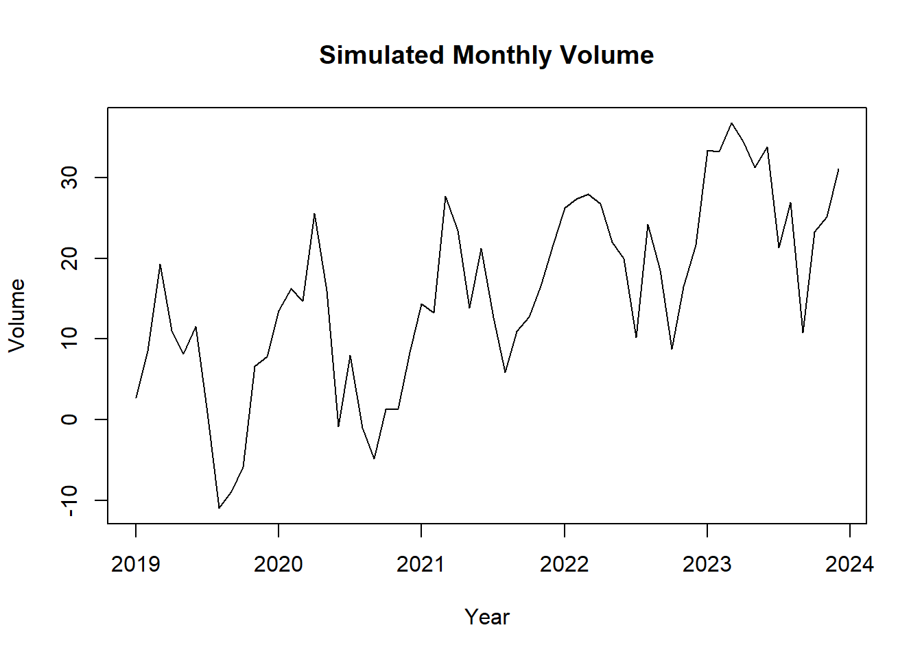

20.15.3 Creating Lagged Variables

volume_vec <- as.numeric(sim_ts)
time_vec   <- as.yearmon(time(sim_ts))

datats <- data.frame(
  Time   = time_vec,
  Volume = volume_vec
) |>
  mutate(
    Lag1 = dplyr::lag(Volume, 1),
    Lag2 = dplyr::lag(Volume, 2)
  )

head(datats, 5)

##       Time    Volume      Lag1      Lag2
## 1 Jan 2019  2.697622        NA        NA
## 2 Feb 2019  8.509367  2.697622        NA
## 3 Mar 2019 19.293542  8.509367  2.697622
## 4 Apr 2019 11.012796 19.293542  8.509367
## 5 May 2019  8.146439 11.012796 19.293542

20.15.4 Scatterplot — Volume vs. Lag 1

ggplot(datats, aes(x = Lag1, y = Volume)) +
  geom_point() +
  geom_smooth(method = "lm", se = FALSE) +
  labs(title = "Volume vs. Lag 1", x = "Lag 1 Volume", y = "Current Volume")

## `geom_smooth()` using formula = 'y ~ x'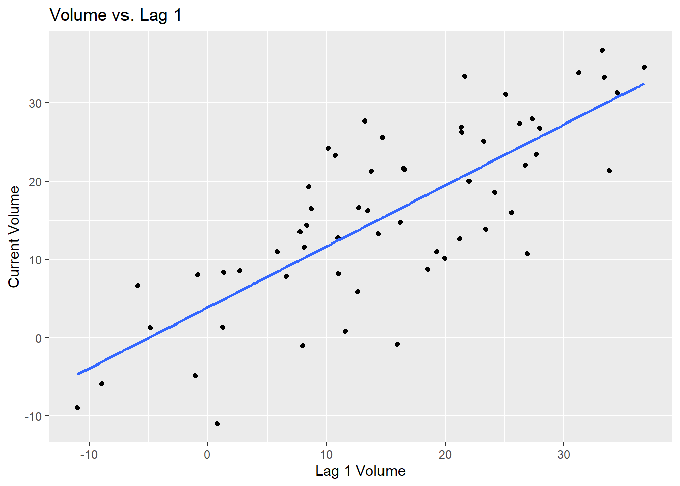

A pattern in this scatterplot suggests the data is good for forecasting.

20.15.5 ACF and PACF

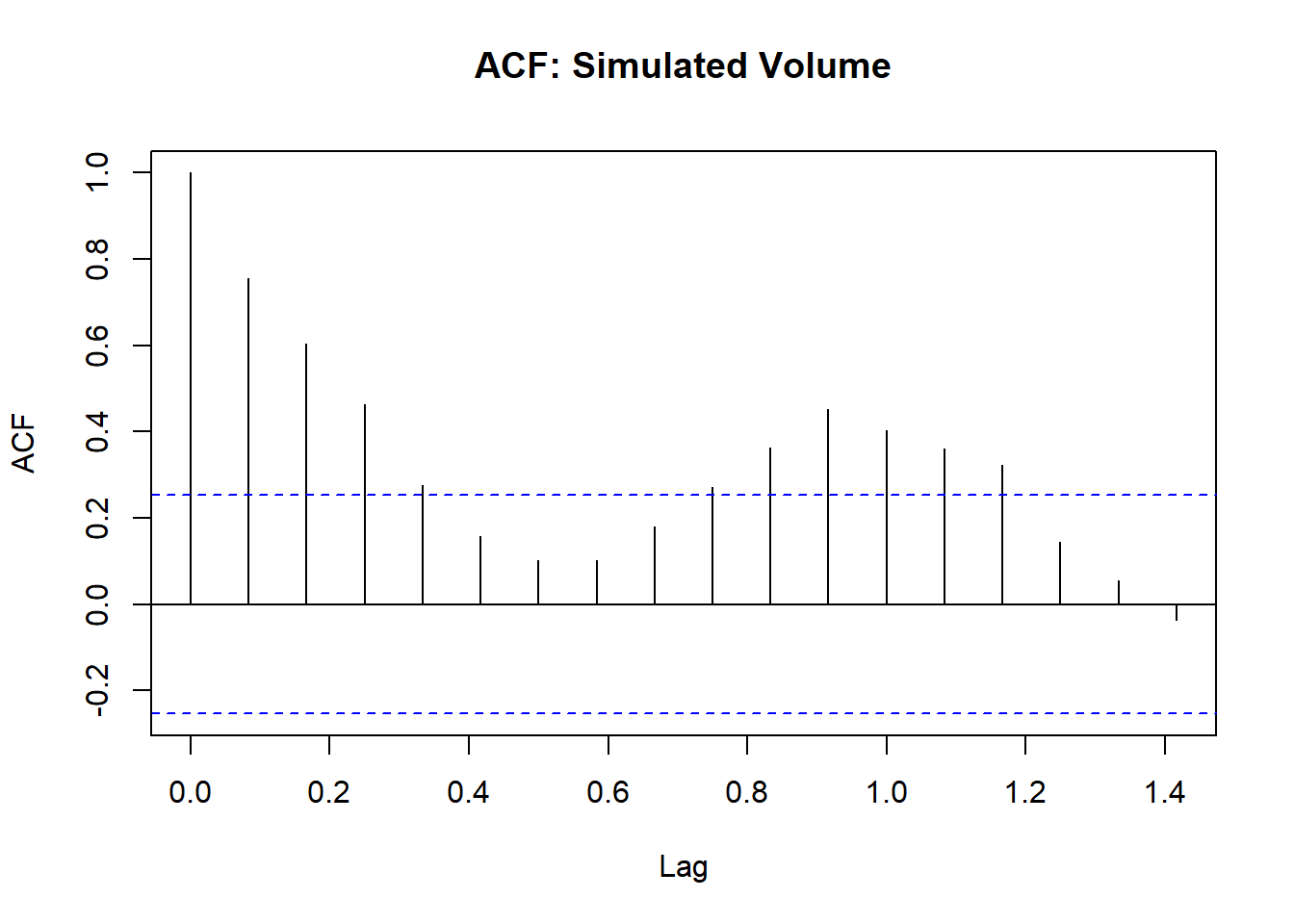
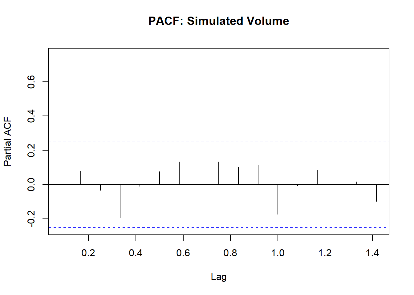
acf(sim_ts,  main = "ACF: Simulated Volume")

pacf(sim_ts, main = "PACF: Simulated Volume")

ACF: Bars crossing the blue lines indicate statistically significant autocorrelation. No sudden cutoff → AR/ARIMA process (not purely MA).
PACF: A spike at Lag 1 with other lags within the blue lines → typical of an AR(1) process.

20.15.6 Stationarity — ADF Test

If p-value > 0.05, differencing is needed.

adf.test(sim_ts)

## 
##  Augmented Dickey-Fuller Test
## 
## data:  sim_ts
## Dickey-Fuller = -5.9266, Lag order = 3, p-value = 0.01
## alternative hypothesis: stationary

20.15.7 `auto.arima`

Automatically selects the best ARIMA(p, d, q) model, checking stationarity, differences needed, and combinations of AR and MA terms.

p: autoregressive order — “if volume was high last month, it may still be high this month”
d: degree of differencing — “what was the movement, increase or decrease?”
q: moving average order — “let me correct based on last month’s prediction error”

tsfit <- auto.arima(sim_ts)
summary(tsfit)

## Series: sim_ts 
## ARIMA(0,0,0)(1,1,0)[12] with drift 
## 
## Coefficients:
##          sar1   drift
##       -0.6482  0.5105
## s.e.   0.1053  0.0445
## 
## sigma^2 = 31.18:  log likelihood = -152.91
## AIC=311.82   AICc=312.37   BIC=317.43
## 
## Training set error measures:
##                      ME     RMSE      MAE      MPE     MAPE      MASE        ACF1
## Training set -0.1763034 4.889015 3.344342 12.61809 63.78359 0.4208828 -0.05025177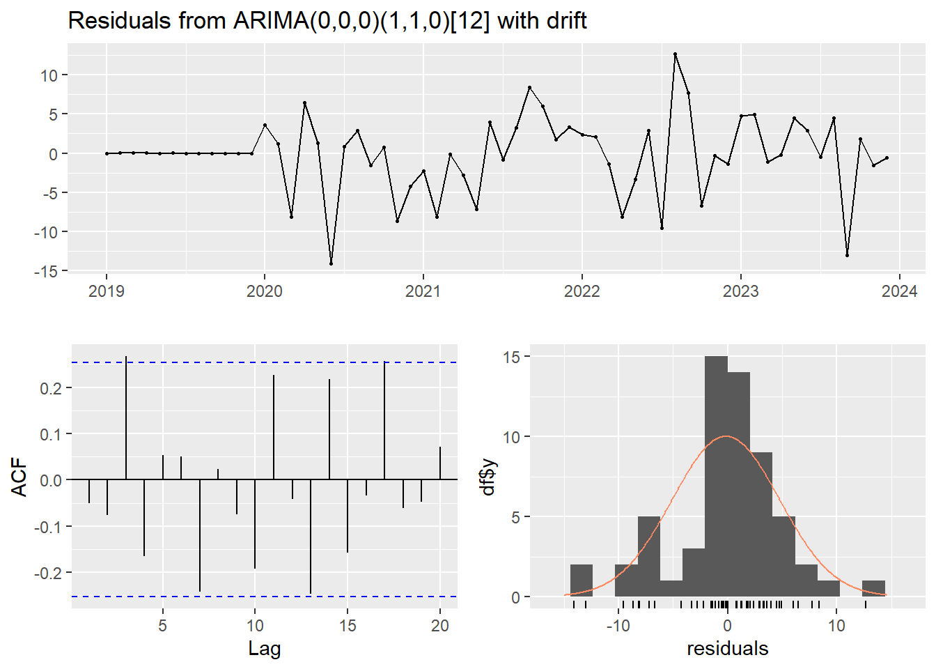

checkresiduals(tsfit)

## 
##  Ljung-Box test
## 
## data:  Residuals from ARIMA(0,0,0)(1,1,0)[12] with drift
## Q* = 18.699, df = 11, p-value = 0.06671
## 
## Model df: 1.   Total lags used: 12

Reading residual diagnostics:

Plot	What you want to see
Residual plot (top)	Random fluctuation around zero, no pattern
ACF of Residuals (left)	All bars within the blue dashed lines
Histogram of Residuals (right)	Normal curve overlaps the histogram

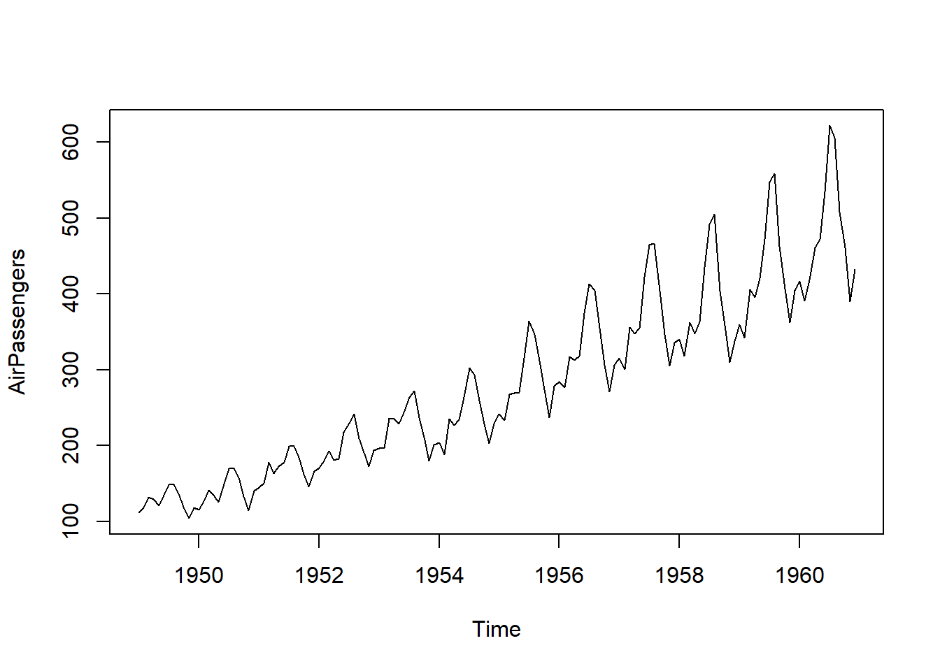
20.15.8 Real Data — AirPassengers

Monthly airline passengers from 1949–1960.

plot(AirPassengers)

datats2 <- data.frame(
  time       = as.yearmon(time(AirPassengers)),
  passengers = as.numeric(AirPassengers)
) |>
  mutate(
    lag1  = dplyr::lag(passengers, 1),
    lag12 = dplyr::lag(passengers, 12)
  )

head(datats2, 15)

##         time passengers lag1 lag12
## 1   Jan 1949        112   NA    NA
## 2   Feb 1949        118  112    NA
## 3   Mar 1949        132  118    NA
## 4   Apr 1949        129  132    NA
## 5   May 1949        121  129    NA
## 6   Jun 1949        135  121    NA
## 7   Jul 1949        148  135    NA
## 8   Aug 1949        148  148    NA
## 9  Sept 1949        136  148    NA
## 10  Oct 1949        119  136    NA
## 11  Nov 1949        104  119    NA
## 12  Dec 1949        118  104    NA
## 13  Jan 1950        115  118   112
## 14  Feb 1950        126  115   118
## 15  Mar 1950        141  126   132

Note: lag12 has no data for the first 12 rows.

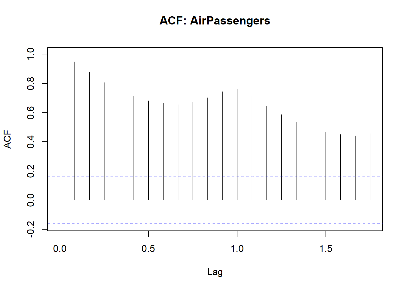
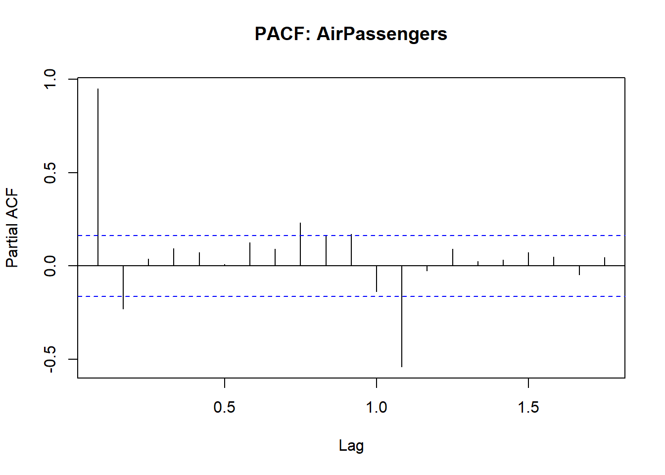
acf(AirPassengers,  main = "ACF: AirPassengers")

pacf(AirPassengers, main = "PACF: AirPassengers")

High autocorrelation at many lags with no sudden cutoff, and a spike at Lag 1 in the PACF, are typical of a non-stationary seasonal series.

adf.test(AirPassengers)

## 
##  Augmented Dickey-Fuller Test
## 
## data:  AirPassengers
## Dickey-Fuller = -7.3186, Lag order = 5, p-value = 0.01
## alternative hypothesis: stationary

Though the ACF/PACF suggest non-stationarity, the ADF may return stationarity due to seasonal effects. Let auto.arima determine the correct differencing.

tsfit2 <- auto.arima(AirPassengers)
summary(tsfit2)

## Series: AirPassengers 
## ARIMA(2,1,1)(0,1,0)[12] 
## 
## Coefficients:
##          ar1     ar2      ma1
##       0.5960  0.2143  -0.9819
## s.e.  0.0888  0.0880   0.0292
## 
## sigma^2 = 132.3:  log likelihood = -504.92
## AIC=1017.85   AICc=1018.17   BIC=1029.35
## 
## Training set error measures:
##                  ME     RMSE     MAE      MPE     MAPE     MASE        ACF1
## Training set 1.3423 10.84619 7.86754 0.420698 2.800458 0.245628 -0.00124847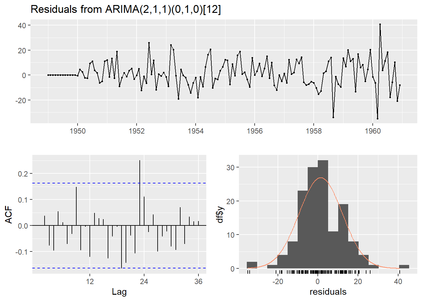

checkresiduals(tsfit2)

## 
##  Ljung-Box test
## 
## data:  Residuals from ARIMA(2,1,1)(0,1,0)[12]
## Q* = 37.784, df = 21, p-value = 0.01366
## 
## Model df: 3.   Total lags used: 24

The best model here is ARIMA(2,1,1)(0,1,0)[12]: trend and seasonality were both present and addressed through differencing. If any bars in the ACF of residuals fall outside the blue lines, consider adjusting the lag terms.

20 Additional Topics

20.1 Preliminaries

20.1.1 Installing and Loading Packages

20.1.2 Datasets Used in This Lecture

20.2 1. Beginning

20.3 2. Causal Inference

20.3.1 Intuition

20.3.2 Econometric Idea

20.3.3 Simple and Multiple OLS

20.3.4 Instrumental Variables

20.3.5 Common Mistakes

20.4 3. Robustness Checks

20.4.1 Intuition

20.4.2 Gradual Addition of Controls

20.4.3 Side-by-Side Comparison

20.4.4 Heteroskedasticity-Robust Standard Errors

20.4.5 Nonlinear Specification

20.4.6 Trimming Outliers

20.4.7 How to read the output

20.4.8 Common Mistakes

20.5 4. Heterogeneity Analysis

20.5.1 Intuition

20.5.2 Econometric Idea

20.5.3 Interaction Model

20.5.4 Separate Subgroup Regressions

20.5.5 Heterogeneity with a Continuous Moderator

20.5.6 Common Mistakes

20.6 5. Moderation Analysis

20.6.1 Intuition

20.6.2 Econometric Idea

20.6.3 R Code

20.6.4 Visualization

20.6.5 Common Mistakes

20.7 6. Mediation Analysis

20.7.1 Intuition

20.7.2 Econometric Idea

20.7.3 R Code

20.7.4 Important Caution

20.7.5 Common Mistakes:

20.8 7. Logistic Regression

20.8.1 Intuition

20.8.2 Econometric Idea

20.8.3 R Code

20.8.4 Common Mistakes

20.9 8. Probit Regression

20.9.1 Intuition

20.9.2 R Code

20.9.3 Common Mistakes

20.10 9. Difference-in-Differences (DID)

20.10.1 Intuition

20.10.2 Econometric Idea

20.10.3 R Code

20.10.4 Manual Check Using Group Means

20.10.5 Common Mistakes

20.11 10. Social Network Analysis

20.11.1 Intuition

20.11.2 Key Concepts

20.11.3 R Code

20.11.4 Common Mistakes

20.12 11. Designing and Testing a Survey

20.12.1 Calculating Sample Size — Proportions

20.12.2 Calculating Sample Size — Means

20.12.3 Testing Survey Reliability — Cronbach’s Alpha

20.12.4 Using a Real Likert Dataset

20.13 12. Panel Data Models (Fixed vs. Random Effects)

20.13.1 Simulated Panel Dataset

20.13.2 Fixed Effects vs. Random Effects

20.13.3 Hausman Test

20.13.4 Real Data Example — Grunfeld Dataset

20.14 13. A Practical Mini Workflow

20.14.1 Mini Practice Flow in R

20.14.2 Careful Interpretation Language

20.15 14. Time Series Forecasting

20.15.1 Lagged Values and Preliminaries

20.15.2 Simulated Monthly Volume Data

20.15.3 Creating Lagged Variables

20.15.4 Scatterplot — Volume vs. Lag 1

20.15.5 ACF and PACF

20.15.6 Stationarity — ADF Test

20.15.7 auto.arima

20.15.7 `auto.arima`